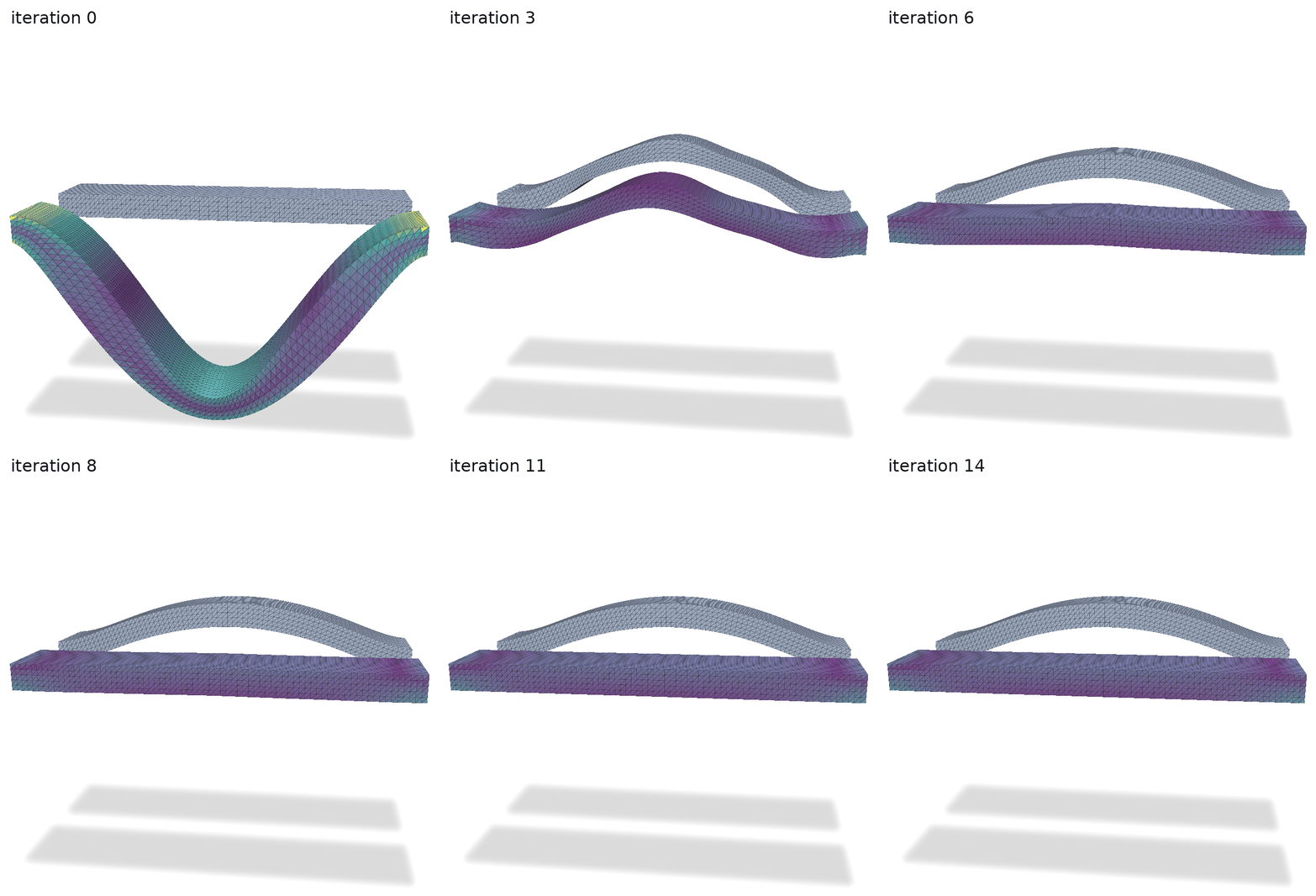
Sensitivity analysis is a powerful technique for optimizing the parameters of a design (e.g., the geometry of a physical object) to achieve a particular goal subject to complex constraints (e.g., under gravity the object should elastically deform to a target shape). I've previously written about the basic mathematical setup for this technique which uses the adjoint method to compute gradients efficiently. I'll try to use the same notation here as much as possible.
As far as I can tell, everything here except the last little trick has already been published in SGN: Sparse Gauss-Newton for Accelerated Sensitivity Analysis by Jonas Zehnder, Stelian Coros, Bernhard Thomaszewski in 2021. So treat this writeup is a rediscovery written in my own words.
Let's consider specifically the problem of rest-shape optimization of a deformable object, where the goal is to deform to a target shape. The rest shape mesh vertices are the design parameters $p \in \mathbb{R}^{3n}$, the deformed mesh vertices $x(p) = p + u(p) \in \mathbb{R}^{3n}$ are computed via displacements $u(p) \in \mathbb{R}^{3n}$, and the target shape is also given as vertex positions $x_\text{target} \in \mathbb{R}^{3n}$.
We'll use a simple quadratic objective function that measures squared error between the deformed shape and the target shape, subject to displacements $u(p)$ being the result of a forward simulation of static equilibrium of the deformable object under gravity. We'll assume that some vertices are fixed to zero displacement (Dirichlet boundary conditions) and the rest are free to move. This can be captured with a sparse Boolean injection matrix $P\in \mathbb{R}^{3n \times 3m}$ (with $P^T P = I_{3m}$) that selects the $3m$ free variables such that $u = P q$ for $q \in \mathbb{R}^{3m}$ spanning the free displacements. We assume that the constrained index set, and hence $P$, remains fixed as $p$ changes.
The whole optimization problem can be written as: $$ \begin{aligned} \mathop{\text{minimize}}_p & \frac{1}{2} \| \overbrace{p + u(p)}^{x(p)} - x_\text{target} \|^2 \\ \text{ subject to } & u(p) = P \left[ \mathop{\text{argmin}}_q \, \frac{1}{2} q^T P^T K(p) P q - q^T P^T M(p) g \right] \end{aligned} $$
where $K(p)$ and $M(p)$ are the sparse linear elasticity stiffness and mass matrices respectively. For now in this simple model, they only depend on the rest vertex positions $p$ (not the deformation $x$). We apply $g \in \mathbb{R}^{3n}$ as the pointwise gravitational acceleration at each vertex, so $M(p)g$ is the corresponding load.
For a given rest shape $p$, the deformed positions must put this inner optimization problem at equilibrium. So, we can replace the argmin-style constraint with the equilibrium conditions derived by setting the gradient of the inner objective to zero: $$ u = P q \quad \text{and} \quad P^T K(p) P q - P^T M(p) g = 0 $$
Naive application of Gauss–Newton would look at the vector-valued residual function: $$ r(p) = x_\text{target} - p - u(p) $$ and substitute the equilibrium constraint to get a function of only the design parameters $p$: $$ r(p) = x_\text{target} - p - P (P^T K(p) P)^{-1} P^T M(p) g $$
Then we'd compute the Jacobian of this residual function with respect to the design parameters $p$ and use it to compute a Gauss–Newton step. $$ p \leftarrow p - (J^T J)^{-1} J^T r(p) $$ where $$ J = \frac{\partial r}{\partial p} \in \mathbb{R}^{3n \times 3n} $$ .
Explicitly constructing this will not work for large problems. Even though $P$,$K$,$M$ are sparse, the inverse $(P^T K(p) P)^{-1}$ is dense implying that $J$ is dense. Matrix-free Jacobian-vector and vector-Jacobian products avoid storing $J$, but each requires a solve with $P^T K P$. A factorization or preconditioner can be reused, making this an important alternative to the sparse direct formulations below.
One cold comfort is that for small problems, doing finite-differences (or forward-mode autodiff) for a gradient $\frac{\partial f}{\partial p}$ requires the same number of seeded forward evaluations as constructing the full Jacobian $J$, though the latter also stores the dense matrix. So if we're prototyping small problems we might as well use Gauss–Newton.
Fortunately, we can avoid constructing $J$ or any dense input matrices entirely. This avoids the quadratic storage of an explicit dense Jacobian, though a sparse direct factorization may still incur fill-in.
Let's rewrite the problem but instead of substituting $u$ with the equilibrium constraint, we will keep the free displacements $q$ as a free variable and add the equilibrium constraint explicitly. The problem is an optimization over $p$ and $q$ as variables: $$ \begin{aligned} \mathop{\text{minimize}}_{p,q} & \frac{1}{2} \| p + P q - x_\text{target} \|^2 \\ \text{ subject to } & \underbrace{P^T K(p) P q - P^T M(p) g}_{R(p,q)} = 0 \end{aligned} $$ where $R(p,q)$ is the residual of the equilibrium constraint.
Consider now $\varepsilon$ perturbations of the rest positions $p$ and free displacements $q$: $$ p(\varepsilon) = p + \varepsilon \delta p, \quad q(\varepsilon) = q + \varepsilon \delta q. $$ Assume that at any given step in the optimization we're at equilibrium, so $R(p,q) = 0$. Then we can compute the total derivative of the equilibrium constraint with respect to $\varepsilon$ and set it to zero: $$ \left. \frac{d }{d \varepsilon} R(p(\varepsilon),q(\varepsilon)) \right|_{\varepsilon=0} = 0. $$
Applying the product rule gives $$ 0 = P^T dK[\delta p] P q + P^T K P \delta q - P^T dM[\delta p] g, $$ where $dK[v], dM[v] \in \mathbb{R}^{3n \times 3n}$ are the (sparse) directional derivatives of the stiffness and mass matrices with respect to the direction $v \in \mathbb{R}^{3n}$. That is, $$ dK[v] = \sum_{i=1}^{3n} \frac{\partial K}{\partial p_i} v_i, \quad dM[v] = \sum_{i=1}^{3n} \frac{\partial M}{\partial p_i} v_i. $$
Using $u = P q$ and letting $A = P^T K P$, $$ A \delta q = P^T (dM[\delta p] g - dK[\delta p] u), $$ and for fixed $u$ the part in the parenthesis is a sparse linear function of $\delta p$: $$ G \delta p = dM[\delta p] g - dK[\delta p] u, $$ where the $j$-th column of $G$ is $$ G(:,j) = \frac{\partial M}{\partial p_j} g - \frac{\partial K}{\partial p_j} u. $$ The matrix $G$ is sparse because perturbing one rest vertex changes only the element contributions incident on that vertex and hence only nearby equilibrium-force entries.
Since we only need the rows corresponding to the free displacements, let's let $$ G_f = P^T G \in \mathbb{R}^{3m \times 3n}, $$ and the linearized equilibrium constraint becomes $$ A \delta q - G_f \delta p = 0. $$
Phew, now, returning to the objective function, we look for $\delta p$ and $\delta q$ that minimize the linearized objective function: $$ \begin{aligned} \mathop{\text{minimize}}_{\delta p, \delta q} & \frac{1}{2} \| p + \delta p + P (q + \delta q) - x_\text{target} \|^2 \\ \text{ subject to } & A \delta q - G_f \delta p = 0. \end{aligned} $$ Using the method of Lagrange multipliers to solve this linearly constrained convex quadratic optimization problem, we introduce a Lagrange multiplier $\lambda \in \mathbb{R}^{3m}$ and form the Lagrangian: $$ \mathcal{L}(\delta p, \delta q, \lambda) = \frac{1}{2} \| p + \delta p + P (q + \delta q) - x_\text{target} \|^2 + \lambda^T (A \delta q - G_f \delta p). $$ and differentiating with respect to $\delta p$, $\delta q$, and $\lambda$ gives the first-order optimality conditions: $$ \begin{bmatrix} I_{3n} & P & -G_f^T \\ P^T & I_{3m} & A^T \\ -G_f & A & 0 \end{bmatrix} \begin{bmatrix} \delta p \\ \delta q \\ \lambda \end{bmatrix} = \begin{bmatrix} r \\ P^T r \\ 0 \end{bmatrix}, $$ where $r = x_\text{target} - p - P q$ and every subblock of the system matrix is sparse. The Gauss–Newton step is then given by $\delta p$, and $\delta q$ is the corresponding change in the free displacements that maintains equilibrium. It can be used to update $q$ alongside $p$, or discarded if the forward equilibrium problem will be solved again after updating $p$.
We can show how the KKT system above is equivalent to the naive Gauss–Newton step by block elimination. Starting with the last row, $$ \delta q = A^{-1} G_f \delta p. $$ Substituting into the linearized objective gives $$ \frac{1}{2}\left\| \underbrace{\left(I+P A^{-1}G_f\right)}_H\delta p-r \right\|^2. $$ Thus the reduced normal equations are $$ H^T H\,\delta p=H^T r, \qquad H=I+P A^{-1}G_f. $$ With our convention $r(p)=x_\text{target}-p-Pq(p)$, the actual residual Jacobian is $J=\partial r/\partial p=-H$. Therefore this is exactly the usual Gauss–Newton equation $$ J^T J\,\delta p=-J^T r. $$
The KKT system is sparse and symmetric, but it's large ($3n + 6m$ unknowns) and indefinite. In our particular setting, the design parameters (rest shape) $p$ enter the residual $r$ directly and rather than minimizing the linearized residual's norm we can directly set the linearized residual to zero, provided the resulting tangent system is nonsingular: $$ p + \delta p + P (q + \delta q) - x_\text{target} = 0. $$ Combining this with the linearized equilibrium constraint gives a square system of equations: $$ \begin{bmatrix} I_{3n} & P \\ -G_f & A \end{bmatrix} \begin{bmatrix} \delta p \\ \delta q \end{bmatrix} = \begin{bmatrix} r \\ 0 \end{bmatrix}. $$ And substituting the first row into the second gives $$ \underbrace{(A + G_f P)}_T \delta q = G_f r $$ which can be solved for $\delta q$ and then $\delta p$ can be recovered via $$ \delta p = r - P \delta q. $$
This matrix $T \in \mathbb{R}^{3m \times 3m}$ is sparse but generally non-symmetric; it is not guaranteed to be positive definite or even nonsingular. So this final "trick" is useful when a robust generic sparse solver (e.g., LU or QR) is available. On the other hand, it won't apply to problems where the residual vector is a different dimension or more complex function of the design parameters where we can't expect there to be a zero solution to its linearization.
As mentioned at the beginning, everything appears already in SGN: Sparse Gauss-Newton for Accelerated Sensitivity Analysis by Jonas Zehnder, Stelian Coros, Bernhard Thomaszewski in 2021. Their treatment is more general: general loss functions, non-linear physics energies (e.g., $K$ is a function of $p$ and $x$). They also show how to add regularizers and take advantage of the block structure of the KKT system in certain scenarios.